10. Example 1: Redshift survey (GMOS-S)

This step-by-step example shows how to create a normal mask for GMOS-S. It is assumed that you have SExtractor installed.

10.1. Creating the OT

First, create a working directory somewhere on your computer, and copy the GMOS-S image and SExtractor configuration files that come with GMMPS into it:

mkdir ~/gmmps_practice/
cd ~/gmmps_practice/
cp /some_path/gmmps-<version>/examples/* .

Second, run Sextractor:

sex -c gmmps.conf NGC7796_GMOS-S.fits -CATALOG_NAME objects_zsurvey.fits

Launch Gemini IRAF in the working directory and open the mostools package:

ecl> gemini
ecl> gmos
ecl> mostools

Convert the SExtractor FITS table using stsdas2objt, so that GMMPS can understand it:

ecl> epar stsdas2objt

intable = objects_zsurvey.fits
image   = NGC7796_GMOS-S.fits
fl_wcs  = yes
instrum = gmos
id_col  = NUMBER
mag_col = MAG_AUTO
x_col   = X_IMAGE
y_col   = Y_IMAGE

This creates the OT table, objects_zsurvey_OT.fits. Launch GMMPS:

gmmps NGC7796_GMOS-S.fits

Adjust the contrast by setting the low / high counts to 1800 and 2500, respectively. Open the objects_zsurvey_OT.fits FITS table: GMMPS -> Load Object Table (OT *.fits)

10.2. Acquisition stars

All objects in the FITS table appear as green squares, meaning they have the default priority 2.

Select three well separated, non-saturated acquisition stars at x/y coordinates 655/388, 2171/399 and 1582/1949. Click on them to highlight the green square, then click on the pink “Acquisition” box. The symbol around the object changes to a magenta diamond (see Fig. 10.2).

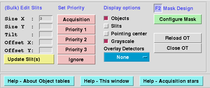
Fig. 10.1 Use the OT window to prioritize targets and adjust slit geometries.

10.3. Prioritize science targets

Assume you want to conduct a redshift survey of brighter field galaxies. Select each object of interest, and click on the pink “Priority 1” button. The symbol around the object changes to a red circle. Repeat until all objects of interest have been set to priority 1.

Note

You may select science objects located in the detector gaps (e.g. the one at 1038/791), because the light gets dispersed before it reaches the detector. However, GMMPS will reject acquisition stars in or very near the gaps because for the acquisition images the light does not get dispersed, and thus the objects will be compromised by the detector gaps.

You can also select all objects of interest at the same time using repeated ctrl-clicks in the image, and then do a final click on “Priority 1”. There is a bug in GMMPS that highlights a much larger number of objects in the OT table display with a yellow background. Make the multiple selection go away by clicking anywhere in the table, or on any object in the field.

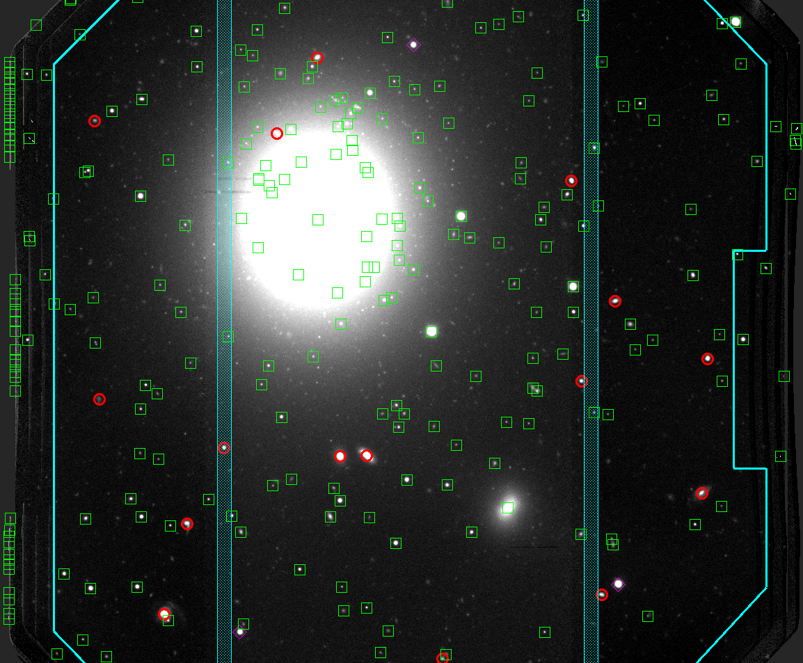
Fig. 10.2 Acquisition stars are shown by magenta diamonds, and priority 1 objects by red circles.

10.4. Adjusting slit geometries

By default, all slits are 1” wide and 5” long. To adjust the slit geometry, select the object(s) of interest, enter the Size X and Size Y parameters under (Bulk) Edit Slits, and then click the yellow Update Slit(s) button. To verify that the slit geometries have changed, you can select Slits under Display Options.

Let’s assume we are happy with the default settings, and particularly interested in the edge-on galaxy at coordinates 935/564. The object is not in the catalog, but its brighter neighbor is (see Fig. 10.3).

Switch on the “Slits” display option. Select the brighter priority 1 neighbor by clicking on the red circle. Enter Offset X = 0.46 and Offset Y = -1.3 (arcsec) to move the slit onto the nucleus of the edge-on galaxy. Due to a short-coming in GMMPS, you must again turn on the Slits display option after each edit to visualize the change.

Change the slit length to Size Y = 9 (arcsec) and the slit angle to Tilt = -8 (degrees) to probe the entire extent of this galaxy.

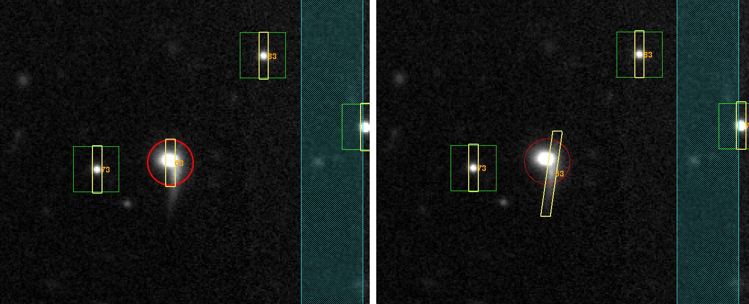
Fig. 10.3 Shifting and tilting a slit

10.5. Making the mask

Click on the green Configure Mask button to launch the final step of the mask design. These galaxies are typically at low redshift, and you expect the most interesting spectral features in the observed 400-600 nm range. Select the B600 grating without filter (Open), and set the CWL to 500 nm.

Select Auto expansion if you want to maximize the sky coverage for each slit. After all slits have been placed on the mask, they will be expanded in length until they come within the Minimum separation (default: 4 pixel) of each other.

GMMPS can decenter the slits length-wise with respect to the objects, to allow for more slits to be placed on the mask. This is controlled by the Auto-finesse parameter, which defaults to 15% of the slit length.

In this example we assume that we are happy with the default settings and a single mask. Click on Make Masks. This will create a single FITS file, objects_zsurvey_OTODF1.fits.

GMMPS now informs you that second order overlap will occur above 665 nm for the B600 grating / no filter combination. You could choose the OG455 order sorting filter to avoid the overlap. However, in this case you would lose the spectrum below 455nm (where you expect some important redshift features), so lets accept the overlap. Close the mask design window and the OT window.

10.6. Displaying the mask

Load the mask design, objects_zsurvey_OTODF1.fits:

GMMPS -> Load Object Definition File (ODF *.fits)

The figure below shows all objects that were included in the mask. Most of the priority 1 objects are present. Some of them, e.g. the two brighter galaxies at 1372/766 and 1479/769 were not placed, because their spectra would overlap with that of the object in the chip gap at 1039/790.

To change this, you could

1. Increase the “Auto-finesse” parameter

2. Give the object in the gap a lower priority

3. Let GMMPS create two masks instead of one

4. Change the position angle. This would require taking a new pre-image with Gemini (time charged to your program). If you are working with a pseudo-image, you could simply recreate the pseudo-image with a different position angle.

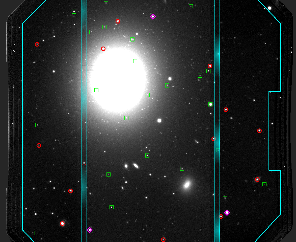
Fig. 10.4 Objects included in the mask design.

10.7. Wavelength overlay

Next, display “Slits & Spectra*. This will show a bunch of information, some of which can be hidden for more clarity:

1. The wavelength interval cut out of each spoectrum by the detector gaps (cyan).

2. A wavelength grid for each spectrum (yellow).

3. Second order overlap (orange shaded region), which appears for objects in the right half of the detector, only.

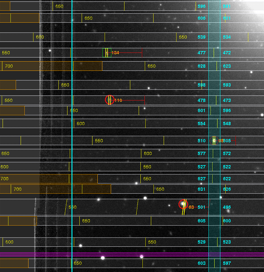
Fig. 10.5 Wavelength overlay. Note the tilted slit in the bottom half.

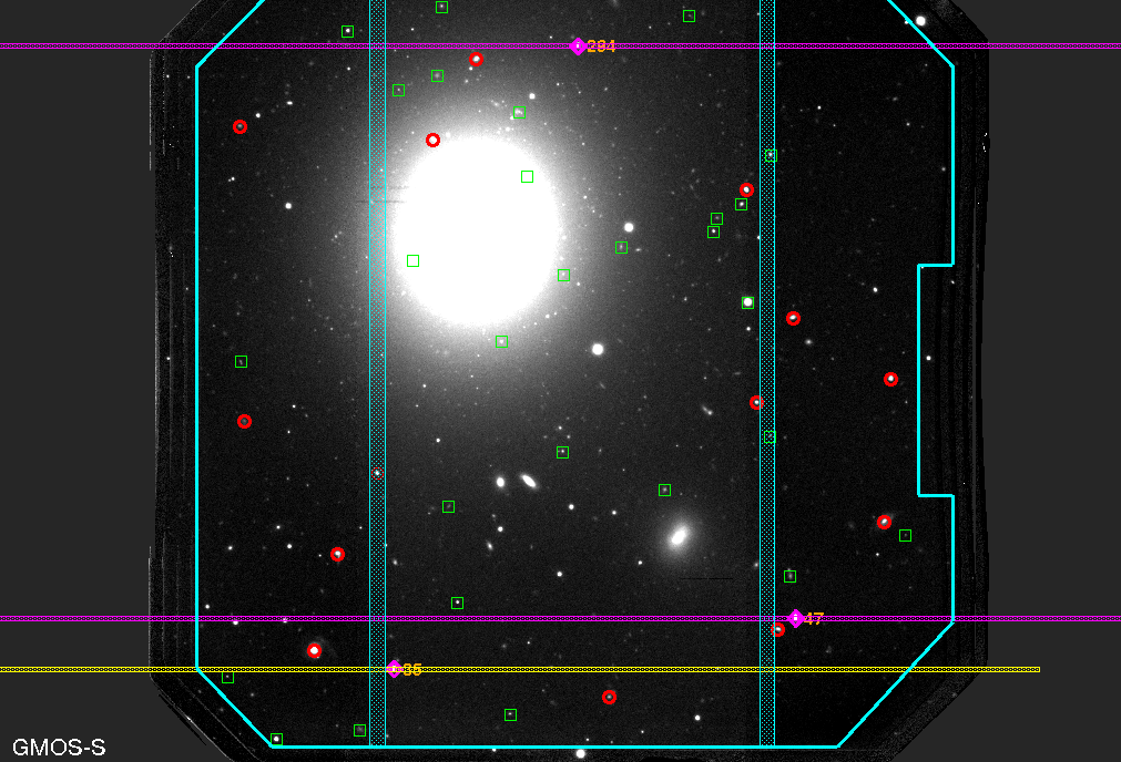
Fig. 10.6 Clicking on “Highlight acq stars” displays the lowest guide star in yellow, meaning it is within 4” of the detector gap (or the boundary of the slit placement area). Most likely, this acquisition star is fine. Since this mask design is based on a GMOS pre-image, the other two (good) acquisition stars will be sufficient to align the mask on sky in case the lowest acquisition star turns out to be problematic. GMMPS will issue an error during mask design if an acquisition star gets too close to a gap or the field boundary.

10.8. Fine-tuning the CWL

Let’s assume you want to verify that most galaxies belong to some cluster at redshift 0.25. The best way to do this would be to look for the prominent [OIII] and [OII] emission lines, and the strong Ca H+K absorption feature.

Enter the atomic identifiers “O Ca” in the field Show other wavelengths [nm] and 0.25 in the Redshift field. The redshifted lines will be overlaid over each spectrum, and you can optimize the central wavelength using the CWL spinbox so that no (or a minimum number of) lines get lost in a detector gap. Alternatively, instead of “O Ca” you could also enter “501 327” if interested in the two brightest oxygen lines, only.

10.9. OT setup and mask submission

Once you activate the Slits & Spectra overlay, GMMPS will also show the relevant phase-II parameters. Make sure you use exactly these values in the Observing Tool.

Lastly, rename the ODF to match your program ID, e.g. GS2017AQ025-01, and upload it together with the pre-image using the Observing Tool’s file attachment facility.

We will review your mask design and contact you if changes are necessary. Otherwise, the mask will be cut, inspected, and stored in our summit mask cabinet. The mask will be installed in the instrument when your observations are scheduled.