11. Example 2: Band-shuffling (GMOS-S)
This step-by-step example shows how to create a band-shuffle mask for GMOS-S. It is assumed that you have SExtractor installed.
11.1. Creating the OT
Now we are interested in the globular cluster system around that large elliptical galaxy. You want to get spectra for a large number of objects in a small region, and therefore the GMOS bandshuffle mode is your best choice.
Compared to the first example, you’d need to detect fainter objects, and further inside the galaxy halo. Create a working directory and copy the test data like for the first example.
Adjust the detection thresholds in gmmps.conf to detect fainter sources:
DETECT_THRESH   = 3
DETECT_MINAREA  = 3
DEBLEND_MINCONT = 0.000001
Run SExtractor:
sex -c gmmps.conf NGC7796_GMOS-S.fits -CATALOG_NAME objects_globclus.fits
Don’t forget to run this table through stsdas2objt as in the first example.
11.2. Prioritizing objects
Launch GMMPS and load the new OT FITS table.
Many objects are present in the OT table, and the view is cluttered. In the dark red top menu bar of the OT window, click on Options -> Set Plot Symbols…. In the table at the very top of the dialog, locate the column called Condition and the entries for $priority == “1” and $priority == “2”. Highlight them, and reduce their symbol size from 15 to 7.
Next, manually click on all your globular cluster candidates and assign them priority 1 (probably you have some multi-color information available that helped you to filter the SExtractor table in first place).
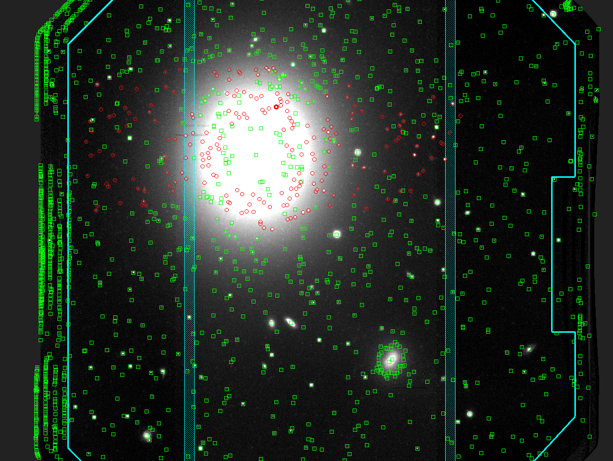
Fig. 11.1 Selection of globular cluster candidates.
11.3. Sorting the OT
You have set the priority to 1, but forgot to decrease the slit length to 0.6” at the same time. In band-shuffle mode, you can use very short slits because the sky will be obtained in separate exposures where the telescope nods to an empty sky position.
Instead of tediously picking all objects again, you can sort the table view in the OT window with respect to the “priority” column:
In the dark red top menu bar, select Options -> Set Sort Columns…. Locate priority under Table Headings, and then press the left arrow to move priority into the “Sort Keys”.
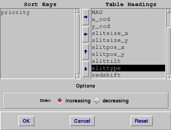
Fig. 11.2 The object table can be sorted.
In the table view of the OT window, scroll to the top where you will find all priority 1 objects. Click on the first, and shift-click on the last priority 1 object to select all of them. Skycat will highlight the selected objects with yellow color, and probably auto-adjust the scroll bar (don’t get irritated by this). Enter Size Y = 0.6 and click on the yellow Update Slit(s) button.
11.4. Define the science bands
Click on Configure Nod & Shuffle Mask. Select Band-shuffle Mode, and set
Band Size (unbinned pix)      = 810
Bands y Offset (unbinned pix) = 50
Shuffle Amt (unbinned pix)    = 810
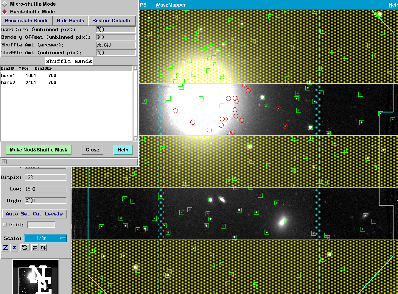
Fig. 11.3 Fine-tune the height of the science and storage bands, and a global starting offset, to match your scientific needs. In this example we want a wide(r) science band on top of the large elliptical galaxy. A storage band at least as high as the science band is required above the science band. If you wanted a very wide science band, you would need to take another pre-image with the galaxy centered in the detector center.
This will define two science and three storage bands. The top science band is centered on the large elliptical galaxy.
11.5. Acquisition stars
Next, we need to find some acquisition stars. These must be located inside the science bands. Let’s pick the stars at 798/1515, 801/593 and 1532/517.
11.6. Mask design
Let’s assume we are interested in a small spectral range only, for example the Ca triplett at 850, 854 and 866 nm, at the galaxy’s hypothetical redshift of z=0.08. We choose the R400 grating and the z+CaT filter combination, selecting a small wavelength range of 830-970 nm. The latter will allow two spectral banks to be mapped next to each other on the detector, so that more slits can be placed at the same time.
For the moment, let’s accept the default CWL of 896nm suggested by GMMPS. Because of the high number of objects, we set Number of Masks = 2 and click on “Make Masks”.
The information window tells us how many objects of each priority were included in the two mask designs. The same three acquisition stars are used in both masks.

Fig. 11.4 Summary of the object types placed in the masks
11.7. Displaying the mask design
The two masks are called objects_globclus_OTODF1.fits and objects_globclus_OTODF2.fits. Load the first one, enter the redshift of the bright elliptical galaxy (z=0.08), and enter “Ca” in the field Show other wavelengths. Set CWL=920 to avoid any of the Ca triplet lines being lost in the detector gaps.
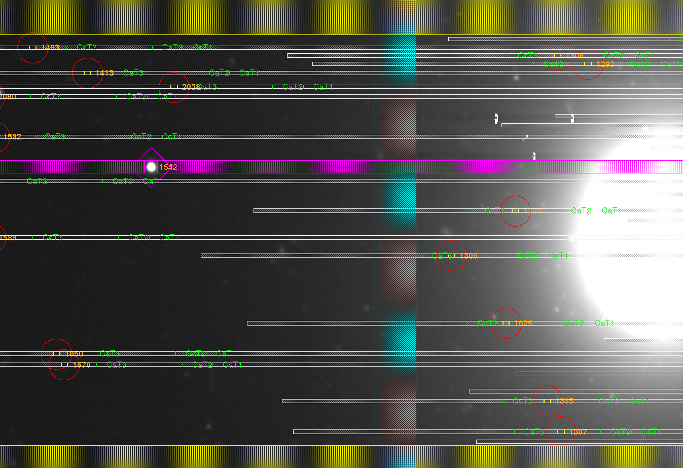
Fig. 11.5 The CWL has been adjusted so that the Ca triplet lines stay clear of the detector gaps.