12. Example 3: Flamingos-2 mask

This step-by-step example shows how to create a mask for F2. It is assumed that you have SExtractor and the Gemini/IRAF package installed.

12.1. Creating the Object Table (OT)

Create a working directory and copy the test data like for the first example, this time using the image N159_F2.fits.

Adjust the detection thresholds in gmmps.conf:

DETECT_THRESH   = 20
DETECT_MINAREA  = 20

Run SExtractor:

sex -c gmmps.conf N159_F2.fits -CATALOG_NAME n159_objects.fits

The necessary Gemini IRAF reformatting tool is located in the gmos package, so we use just that like in the first example. Launch IRAF, and therein

ecl> gemini
ecl> gmos
ecl> mostools

Convert the SExtractor FITS table using stsdas2objt, so that GMMPS can understand it:

ecl> epar stsdas2objt

intable = n159_objects.fits
image   = N159_F2.fits
fl_wcs  = yes
instrum = flamingos
id_col  = NUMBER
mag_col = MAG_AUTO
x_col   = X_IMAGE
y_col   = Y_IMAGE

Executing stsdas2objt will produce the OT n159_objects_OT.fits that can now be used by gmmps.

12.2. Acquisition stars for mask alignment

Launch GMMPS as

gmmps N159_F2.fits

and adjust the brightness level using 1600 and 1900 for the low and high thresholds, respectively.

Load the OT table from the main menu:

GMMPS -> Load Object Table (OT *.fits) -> n159_objects_OT.fits

Select three non-saturated acquisition stars at (x/y) = 475/1227, 1237/817 and 1843/1075, which are well separated and yet do not interfere too much with the placement of the science slits. By clicking the “Acquisition” button below “Set priority”, the selected stars will become acquisition stars with the highest priority for mask design and assigning to each a 2x2 arcsec box.

12.3. Sky subtraction

Before moving on to the actual mask design you must decide on a sky subtraction strategy. While this is also of some relevance for optical spectra with GMOS, it is paramount in the near-infrared with F2. There are two options:

1. Use the default slit length of 5”, which allows for sufficient sky coverage in case of compact objects, and use a ABBA nodding pattern within the slit. Note that in case of tilted slits you must use a nod offset, as otherwise both nod offsets will drive the object off the slit.

2. Nod the telescope to a nearby blank sky area, which is required for extended targets (large galaxies, nebulae) were blank sky samples cannot be included in the mask design. While this lowers the effective “on-source” time (compared to nodding within the slit), it offers the opportunity to use very short slits and therefore increase the slit density significantly.

In our example we must choose the 2nd approach because of the extended nebulosity. Of course it is possible to extend some of the slits into nearby sky areas a few arcseconds away, but in general that is not possible for all slits.

Note

To nod within a F2 slit you must use a non-zero p-offset, because the F2 slits are aligned with the detector rows (dispersion is along the vertical axis). For GMOS, you would use a non-zero q-offset, because the slits are aligned along detector columns. The (p/q) coordinate system used for nodding the Gemini telescopes is defined such that p-offsets run along the horizontal detector axis, and q-offsets run along the vertical axis.

12.4. Target selection

In this case we have to nod to a blank field for sky subtraction. Hence, we use 3 arcsec long slits and achieve a higher slit density. Select all slits in the OT window using shift-click, and enter

Size X = 3

followed by Return or a click on Update slit(s) (see also the following Fig.). Our selection also included the three acquisition stars. GMMPS will not change their slit geometry, which is fixed to arcsec square boxes with zero tilt angle.

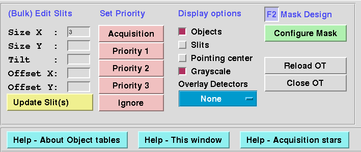
Fig. 12.1 Prioritizing targets and adjusting slit geometries in the OT window.

In this example we arbitrarily select some of the brighter knots in the nebulae: click (or shift-click if you want to select several at once) on the green squares in the image display, and then on the pink Priority 1 button.

For the lower right compact nebula, we use shorter slit lengths of 1.5 arcsec. For the brighter knot near the top of the center nebula at x/y = 1130/1263 we use a 12 arcsec long slit with a tilt angle of 25 degrees.

GMMPS may fill the rest of the mask with objects arbitrarily selected from the priority 2 list.

Fig. 12.2 Prioritized OT table for the F2 mask. Objects outside the cyan slit placement area are not available for the mask design.

Click the green “Configure Mask” button to start the mask design.

12.5. Configuring the F2 mask

The mask configure dialog is shown in the Fig. below:

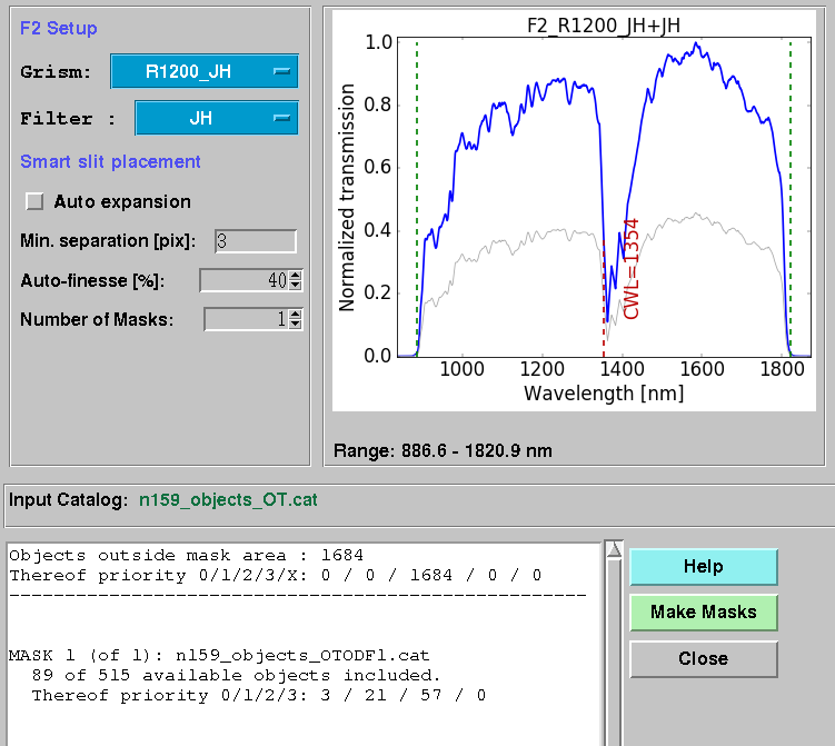
Fig. 12.3 Selecting the optical setup and fine-tuning the slit placement. The solid blue line in the upper right panel shows the relative throughput, the thin grey line the (approximate) absolute throughput.

We choose the low resolution R1200_JH grism with the JH bandpass filter. This will provide full wavelength coverage from 900-1800 nm, as shown by the throughput plot.

We do not auto-expand the slits (applied after all slits have been placed on the mask) because we use separate sky offsets. It does not hurt to use the auto-expansion, though.

The default minimum slit separation in the spatial dimension is four pixel, which is a conservative estimate that allows for robut automatic identification of the spectral footprints. In this example we want to allow for a somewhat tighter packing of slits and choose a minimum separation of 3 pixels. In principle, one could go as low as zero pixels, but then one would have to manually define the spectral traces when reducing the data.

We let GMMPS offset the slits by up to 40% of their length (auto-finesse), to allow for more slits on the mask. Note that for the first sky subtraction method you want the objects to remain at the center of the slit and therefore an auto-finesse of zero must be chosen. We are happy with a single mask.

Upon clicking the green Make Masks button, the slits will be placed on the mask according to their priorities. GMMPS informs us that 515 objects are available in the slit placement area, 89 of which were placed on the mask: 3 acquisition stars, 21 high priority targets, and 57 other objects.

The system will alert you if you have chosen stars with a high proper motion (>100 mas/year) as acquisition stars. While these are OK to use for recent preimages, they should not be used when the mask is designed from a catalog.

Note

Unlike GMOS, F2 uses fixed optical configurations that do not allow adjustment of the central wavelength. Therefore, spectra cannot be moved around on the detector. The most commonly used configurations are therefore the ones that provide maximum spectral coverage, i.e. the R1200_JH and R1200_HK grisms with the JH and HK bandpass filters, respectively, and the R3000 grism (using either Y, J, H or K filters). All of these configurations use most of the F2 detector extent in the spectral direction, and therefore have no impact on the mask design (i.e. which slits are placed). The only exception would be if you use a combination that produces a shorter spectrum, e.g. the J, H or Ks filters with the R1200 grisms. In that case, up to two spectra can be packed in the dispersion direction (see the Fig. at the very bottom).

12.6. Displaying the mask design

Load the mask designs using GMMPS -> Load Object Definition File (ODF *.fits) -> n159_objects_OTODF1.fits

The mask design is visualized in the Figures below.

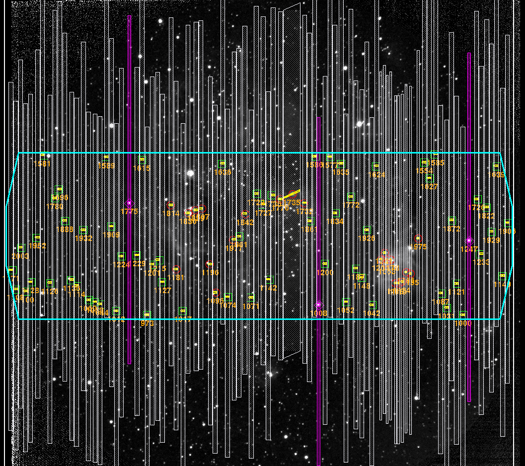
Fig. 12.4 Objects selected for the R1200_JH grism and JH filter combination. Most of the detector array is used to map the spectra.

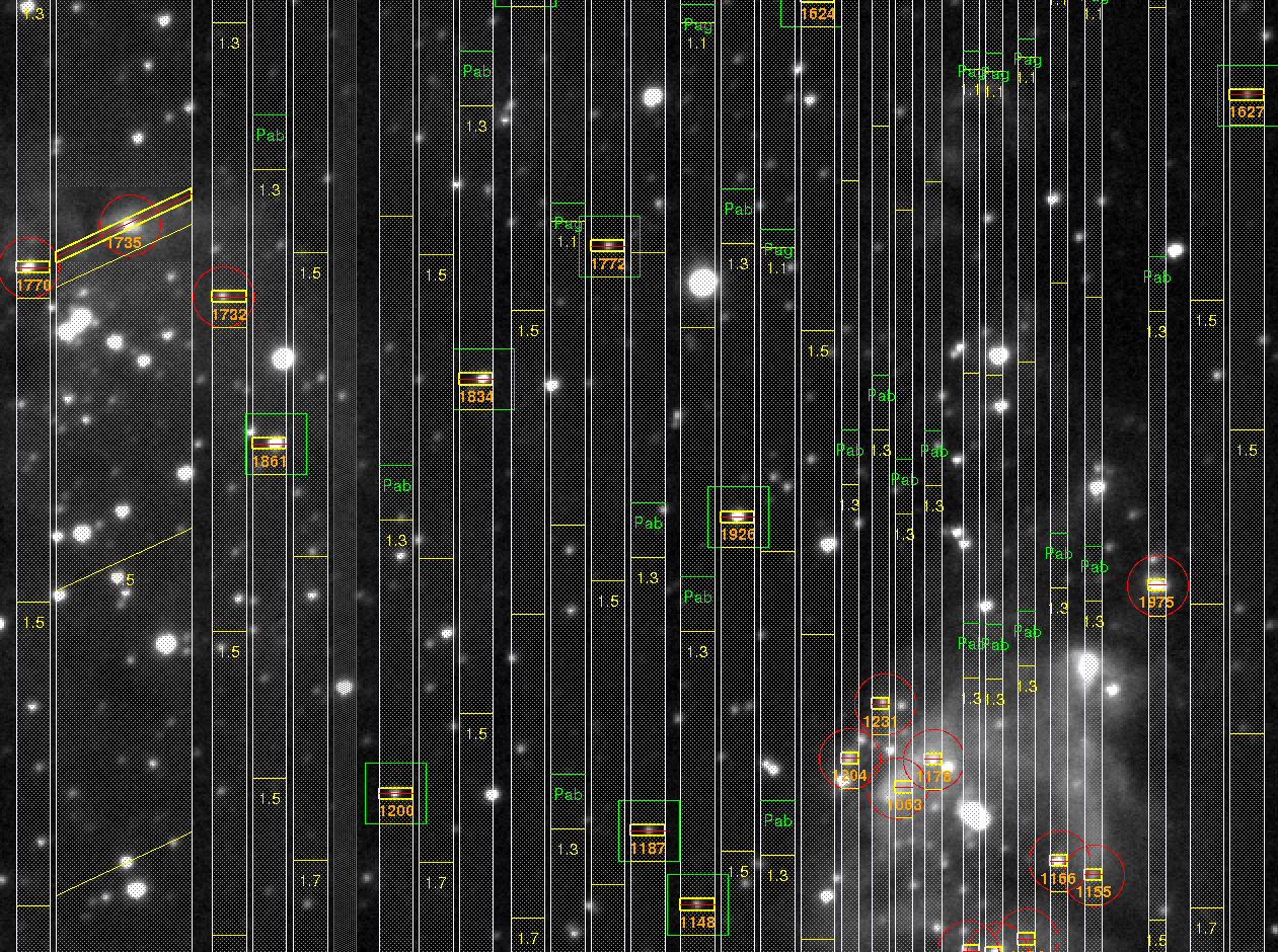
Fig. 12.5 Zoom in on the F2 mask design. Looking at the yellow slits, we recognize that GMMPS offset the slits with respect to some objects to allow for more slits to be placed (e.g. the slit to the right of the tilted spectrum). The wavelengths (yellow numbers) are shown in microns, increasing from top to bottom. We also entered the atomic identifier “H” in the field “Show other wavelengths”, and GMMPS shows the locations of the Paschen Beta and Gamma lines.

Fig. 12.6 Using the J instead of the JH filter, significantly shorter spectra are produced and GMMPS may place up to twice as many slits on the mask (in this case, 140 slits).

Once you are happy with your mask, it is useful to go through the mask checklist to ensure consistency with observing tool information, among others.